About Excel
As a preface, you should note that Excel is a terrible choice of software to do data analysis with. It's fine for planning a family budget, or keeping track of grades, but when it comes to data analysis there are much better choices out there. However, it's what we have right now...
Simple Curve Fitting with Excel
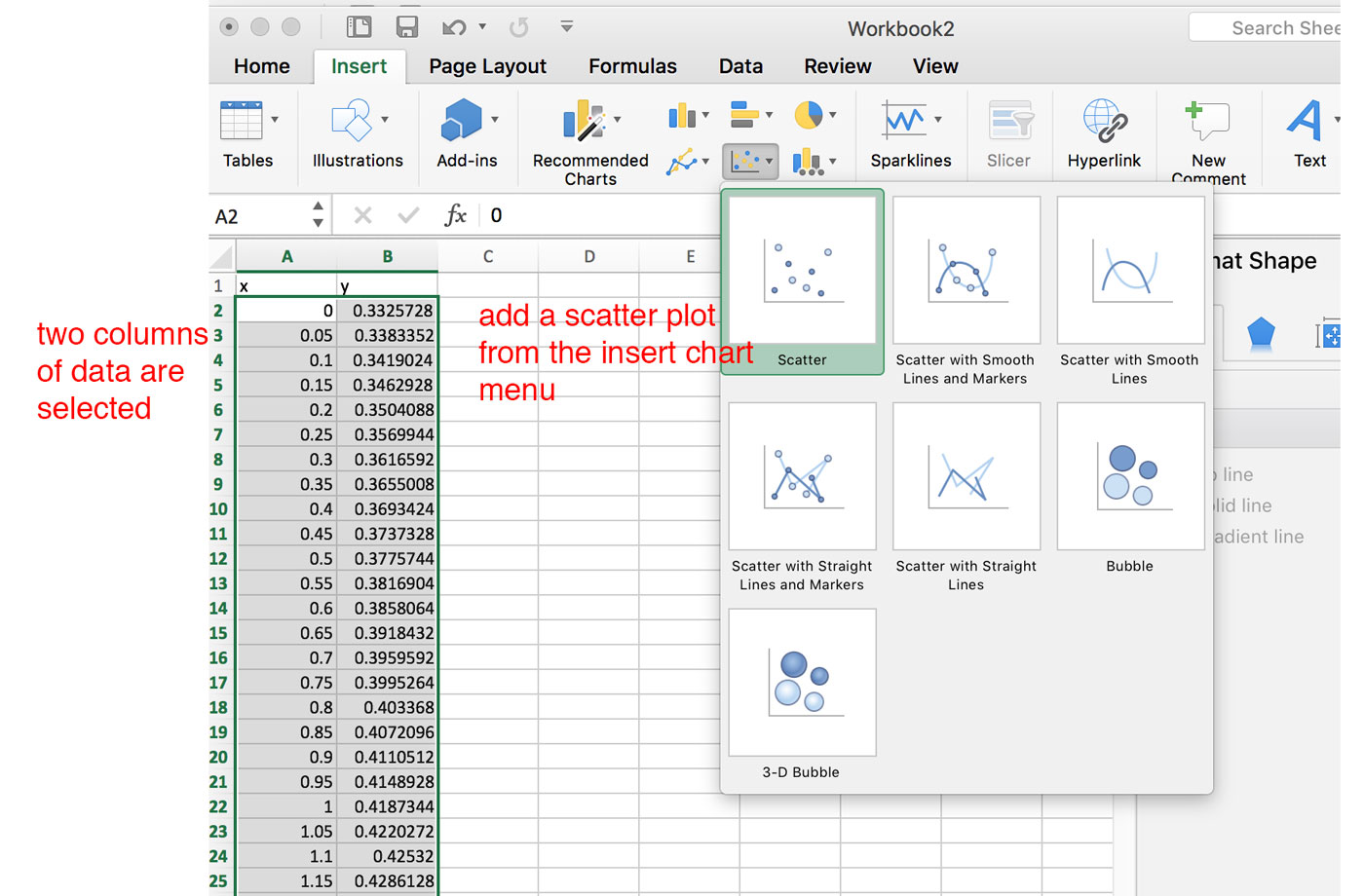
1) To fit a curve in excel, you should begin with two columns of data. We'll call them x and y. Select both columns, then go to INSERT -> CHART -> X Y (scatter)
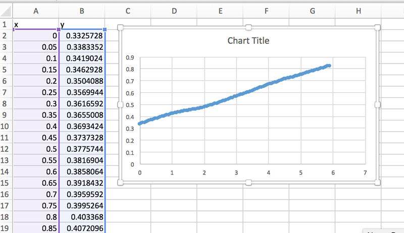
2) After doing this, you'll end up with a chart! On the bottom axis are the x values, and on the left axis are the y.
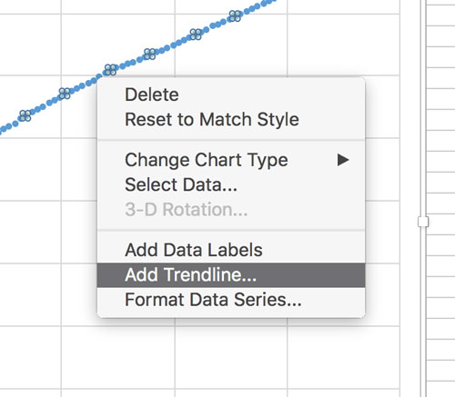
3) Next, right click on the data series (the dots) and you should see an option to "Add Trendline". Do it!
4) After adding a trendline, you should see it behind the data points.
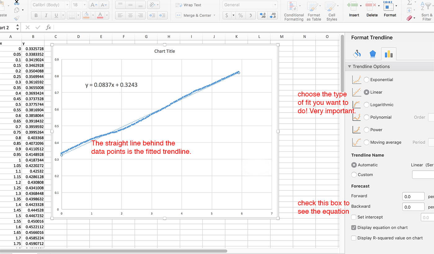
5) You can select which type of function you want to fit with. Also make sure to select the box that says "Display equation on Chart" otherwise, you won't be able to see the values of the function that created the trendline. Read more about functions and fitting here.
Derivatives of a data set
The basic idea of a derivative amounts to finding the change in one variable with respect to another.
Here is an example. Let's take some data for a freely falling object. It starts falling at t=0, and we record its position every second after. We can put this data into two columns in Excel, then plot distance as a function of time. We see the expected parabolic shape.

Let's say we now want to figure out the derivative of position with respect to time: $\frac{dy}{dt}$. If we knew the functional relationship between y and t, this would be easy. $$y = -\frac{1}{2}gt^2 \Rightarrow \frac{dy}{dt}=-gt$$. However, we are working with data points, and not a function. Thus, we have to do a numerical derivative. We can't actually set our $\Delta t \rightarrow 0$, so we'll have to approximate it.
We'll have to manually figure out the change in height (our y variable), with respect to time. Something like the following should suffice. $$y' = \frac{\Delta y}{\Delta t} = \frac{y_1-y_0}{t_1-t_0}$$
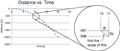
Below is a picture showing this calculation in the Excel sheet. The cell D3 is calculated using the formula =(B3-B2)/(A3-A2). All the subsequent rows in that column are just the same formula applied to next rows down. The cells in column C are just the midpoints between the times used in the calculation.
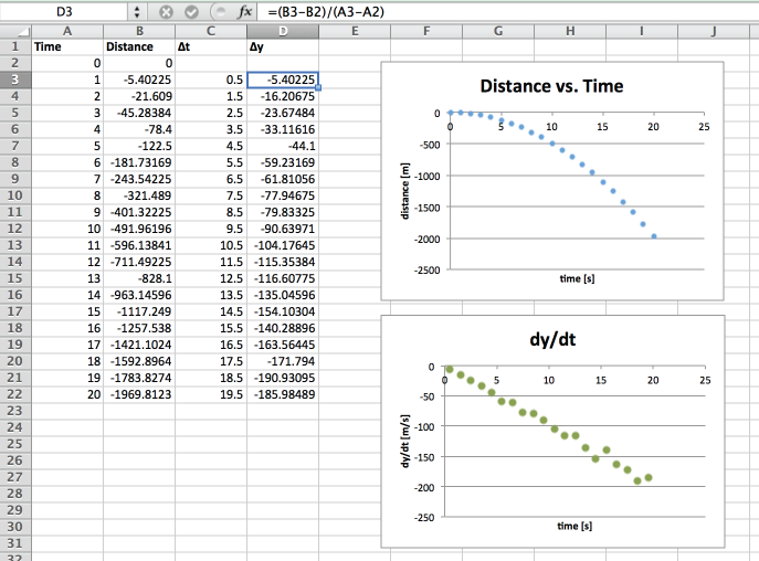
We are essentially finding the slope between each point in the position graph, then plotting those slopes as a function of time. Since the slope of the position w.r.t. time is velocity, we now have a velocity graph. For example, between 10 and 11 seconds, the position changed by -104.2 m. This tells us the velocity at that point (t = 10.5) will be approximately -104.2/1 = 104.2 meters, as shown in the zoom in below. Looking at the velocity graph, we can see that this indeed is the case. The velocity at 10.5 is about 100 m/s.
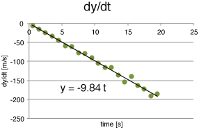
Lastly, we would like to find the slope of the velocity graph in order to determine the free-fall acceleration of this object. For this, we can use the linear fit tool, as shown below. Indeed, we recover an expected 9.8 m/s2.
This is just the most basic way to perform a numerical derivative. There are more thorough methods which you may explore later on.