Physics 103 - Lab 3 - Little g
Introduction
In this lab, we will use several methods to measure the acceleration of an object due to gravity. These methods will be compared for the effectiveness and precision.
The acceleration due to gravity is usually considered to be 9.8 m/s2. This value can be obtained from Newton's universal law of gravitation:
$$F_G = ma = mg =\frac{G M_E m}{r_E^2} \Rightarrow g = \frac{G M_E}{r_E^2}$$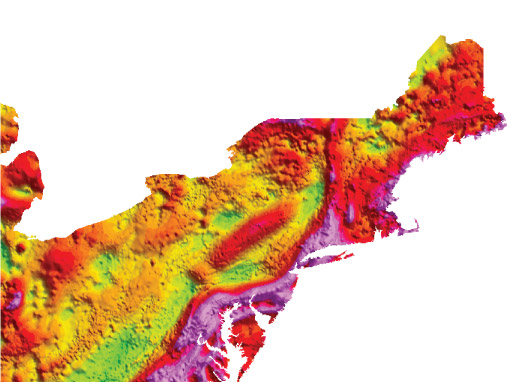
Image source: USGS Geophysics
If we knew the gravitational constant $G$, the radius of the earth, $r_E$, and the mass of the earth, $M_E$, then we could calculate $g$ easily. However, due to differences in the composition of the earth, $g$ is not actually the same everywhere. In fact in New York, it's 9.802 m/s2, but in Los Angeles, it's only 9.796 m/s2 [ref]. This is not a noticeable difference to us in our daily lives, but for some precision applications it could be very noticeable. The image below shows the gravitational anomalies of the North-East US. The variations shown are less than 1% of $g$, but depending on your application this could be a big deal.
Thus, we'll investigate some different ways of measuring $g$.
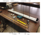
Equipment check
Please make sure your station has all of the following items. If not, check again, then talk to your lab instructor.

Experiment: A rough measurement
First, we'll drop a wooden block from 1 meter and see how long it takes to hit the ground. Since for an object in free fall, $\Delta y = -\frac{1}{2}gt^2$, if we can measure $t$ and $\Delta y$, then we can get a value for $g$. Go ahead and let the wooden block drop from 1 meter high while timing the fall with the stopwatch. Have one person do the dropping and the other do the timing. Do it 3 times and record the three values below.
Find the average of your three measurements and enter it in the box below.
You will no doubt have observed that this is not a very good way to measure $g$.
Report Questions
Why is this method not very good? What are the limitations?
Experiment: Slo-mo free fall
Below is a video recorded in 60 frames per second (fps) of a ball dropping in free fall. Use the frame by frame buttons to measure the distance traveled in some amount of time (your choice). The scale on the wall is in centimeters. You'll need to figure out how much time passes between each frame which you can do if you know if there are 60 frames per second on the video.
After you've measured the distance and time via the video, calculate a value for the free fall acceleration $g$ based on this analysis.
Experiment: Leveling a ramp.
From the previous two measurements, you've hopefully noticed that measuring little $g$ is not a trivial measurement. To get anything better than two significant figures, we'll need to improve our experimental approach.
In lecture, it was shown that a frictionless object sliding down an inclined plane will undergo constant acceleration at the rate of $$a = g \sin \theta$$ where $g$ is the standard acceleration due to gravity, 9.8 m/s2, and $\theta$ is the angle between the ramp's surface and the horizontal plane of the ground.

On the bench is a low-friction track and car. We'll use these to measure $g$ next.
The first step will be to make sure we can accurately know the angle $\theta$ we are dealing with on the ramp.

From the schematic above, we can see that the angle of $\theta$ should be given by $ \theta = \sin^{-1}\left( \frac{h}{L} \right)$. The lengths of our track, $L$, is 122 cm, or 1.22 m.
First, set up the track so that it is level. Use the thumb-screws on each end to make the track level. (i.e. $\theta = 0$) A car placed on the track in this condition should not move. ($a = g \sin \left( \theta \right)= 0$) Verify that you can indeed obtain a $\theta = 0$ track.
Report Questions
Let's consider how 'level' this track really is. Using uncertainty analysis, what is the uncertainty in the angle measurement of the track? Based on this uncertainty, our tracks are probably not exactly at $\theta = 0.000...$. In an ideal physics set up, even a very small angle $\theta$ should create an acceleration. So, why can you get the car to stand still? (here are some tips on uncertainties: Error Analysis)
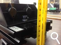
Now, lower the end with the stopper until the cart begins to move. Record the height difference between the two ends and use the trigonometry above to convert this to an angle.
Here is an image that shows how to make this measurement. (Click to zoom in)

Enter this angle in the box below.
Report Questions
Based on this angle, estimate the static (or rolling) friction coefficient that is acting on the car when it's on the ramp. The mass of the cart is ~ 500grams. Essentially, what is the force that prevents it from rolling even if this track is not perfectly level. Include a free body diagram and use Newton's 2nd law with a Sum of forces to explain your calculations.
Experimental Setup: The Rolling Cart
Now, we will let a cart roll down the ramp and record the position as a function of time using the electronic position sensor. The position sensor measures the location of the cart at regular time intervals. The general idea will be to measure the position as a function of time for several different set-ups, in order to obtain another measurement of $g$. Before beginning, make sure to level your track again.
Set up the electronics
- Make sure the data acquisition components are set up correctly, as shown in the picture.
- Open the application LoggerPro3. It should be on the desktop or the taskbar.

Taking Data
The device works by emitting sound waves, (above your hearing range) and measuring how long it takes for them to bounce off the target and return to the device. Since we know the speed of sound, this can be used to calculate a position for the object. The software and electronics do all this work for you, giving you a nice table of data showing time and position. Experiment with acquiring a few data runs before beginning the next section. You'll want to get comfortable with the software before using to do any science. You should use the experiment file called simple-position.cmbl. It should start by default, but if not, here is a copy of it that you can download.
Specifically: make sure you ...
- understand how the different runs are acquired/saved/erased.
- can bring your data into Excel. The easiest way is to just copy the columns from the table on the right of the screen, then paste them into an Excel file. This way, you can trim the selections to only include the data you want. Or, you can save your run files as csv, then import them to Excel. Either way, make sure you can do this reliably.
- can verify the acquisition parameters (time steps, etc). These are set in the top menu: Experiment → Data Collection. For example, you can change how long data is acquired for and how many times per second it acquires the data. (20 samples per second should be enough)
- Try putting your hand in front of the sensor while it is collecting data. Double check that the graphs you see make sense.
You'll use this software later in the term, so it's worth getting familiar with. You can find a manual for it here: LoggerPro 3 Manual (**Always a good idea! Chances are good that in your first job or internship, someone will say: "Go figure out some piece of software or equipment and do this and that with it and report back..." Sometimes there won't even be a manual!**)
Experiment: The Rolling Cart at different angles
The first runs we'll do will be to measure the position of the cart as it rolls down the ramp. The variable we'll be adjusting is the angle of the ramp. Before adding spacers to change the angle, make sure the ramp is level without any spacers.
- Start with one spacer under the side with the motion detector. Measure the height difference between the two ends of the ramp using the ruler, and use the trigonometry described above to calculate the angle $\theta$ of the ramp.
- Place the cart on the raised end of the ramp and get ready to begin the data acquisition via the computer.
- Press the start button, wait a second or two until the clicking sound begins, then release the cart from rest.
- Don't worry about starting and stopping exactly when you let go - you can trim the unwanted data points later.
- Repeat this measurement for three different angles.
Your acquired data for one run should look something like the following:
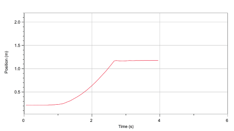
If there are funny looking spikes in the data, adjust the position of the motion sensor slightly until you get a smooth curve.
Make an excel spreadsheet that you will use to analyse this data. Trim your data in Logger before copying into Excel. Look at the table of data points and try to determine when the cart begins to move, and when it stops. Times before you let go, and after it hits the end of the track can be discarded (select the ones you don't want, then use the Edit->Strike Through Data Cells menu item. )

Save your excel spreedsheet with the data from these experiments. You will use it to answer the report questions.
Enter your three angles here.
Report Questions
Your task is to obtain a value for $g$ based on the measurements. You'll need to know the angle for each run so make sure you've carefully noted that variable.
The procedure will be to import the position data into excel, and use the excel curve fitting tools (aka a trendline) to analyse the data. We'll also use the $a = g \sin(\theta)$ relationship to obtain a value for $g$.
If you're not even sure where to begin, here is a quick introduction.Here is an example of what your graphs should look like.
For each angle, perform the analysis separately. Do the three measurements all produce similar results for $g$? Why or why not? Comment on reasons why they might be different.
Experiment: The Rolling Cart with different masses
The next runs we'll do will be to measure the position of the cart as it rolls down the ramp. The variable we'll be adjusting is the mass of the cart.
- Start with one spacer under the side with the motion detector. Measure the height difference between the two ends of the ramp using the ruler, and use the trigonometry described above to calculate the angle $\theta$ of the ramp.
- Place the cart on the raised end of the ramp and get ready to begin the data acquisition via the computer.
- Press the start button, then release the cart from rest. You should hear some clicking and see the position being measured on the display.
- Now, set the four silver rods into the cart as the picture shows.
- Repeat the measurement with the cart+mass

Report Questions
Doing a similar analysis to this data as you did in the question above and determine the acceleration of the cart with and without the mass. Use your analysis to make a claim either that the mass affected the acceleration or that it did not. Would you expect it to based on our understanding of kinematics?
Discrepancies
Now, refresh the table below. It should show a list of the various measurements other groups obtained for the value of $g$ using the slo-motion video earlier in the lab. Copy this table into an excel file, or record it in your notebooks. You will use it to answer the following report questions.
Report Questions
More than likely, there are differences between some groups' estimation of $g$ shown in the table above. Comment on these discrepancies. If everyone had access to the same raw data (i.e. the video), shouldn't their results be the same? What could lead to variations in these results? Calculate the average value from $g$ based on these measurements. Is it within the uncertainty you would expect from the experiment?